15. Simplified Guide to Optimizing Lens Constant Values of Intraocular Lens Power Formulas for Clinicians
Lens constants should be updated whenever there is a change in the intraocular (IOL) type, material, biometer, or surgeon, and once established, should be routinely fine-tuned for optimal results. The significant enhancement of refractive outcomes largely relies on the crucial process of lens constants optimization. Before embarking on any study that explores the accuracy of IOL power calculation – that is, how closely the predicted refraction using a certain IOL power aligns with the actual postoperative refraction -, it is essential to undergo the initial step of constant optimization.
The process of constant optimization using the published 3rd generation formulas – Haigis, Hoffer Q, Holladay 1, and SRK/T – in Excel can be quite laborious. Each eye requires individual formula calculation on a spreadsheet. While you can begin with the manufacturer-provided constant, an optimized value for the group, resulting in a zero mean Prediction Error (PE), must be computed after several cases. The « Goal Seek » function in Excel then has to be used to adjust the formula’s lens constant for each eye to make the calculated mean PE equal to zero, which results in an optimized value for aspects such as pACD (Hoffer Q), Surgeon Factor (Holladay 1), a0 (Haigis) and A-constant (SRK/T). This method, while effective, involves a significant amount of repetitive and meticulous work.
The task of optimizing unpublished formulas, such as Barrett Universal II, EVO, Kane, and Olsen, becomes more complicated as it cannot be achieved solely with Excel. You are left with two choices: either reach out to the authors and request them to do it for you or use particular computer programming languages like Python, which can autonomously pull data from any database, input it into the formula website, and create a new database with the predicted refraction for each eye. The latter option, while possible, requires considerable technical expertise and makes the process even more complex and time-consuming.
This page is dedicated to a new simplified method for obtaining an optimal constant value for an intraocular lens (IOL) in formulas using a single optimization constant. It is accessible to any surgeon wishing to have the ability to adjust the constant value of an IOL for formulas such as SRK-T (A-constant), Haigis (a0), Hoffer Q (pACD), Holladay (SF), Barrett (A-constant), EVO (A-constant), Kane (A-constant) and PEARL-DGS (A-constant).
There is no theoretical obstacle to adapting this method to optimize ray-tracing procedures that use a constant (for example, C constant, Olsen formula).
If optimization and the concept of constants are not new to you, feel free to skip the following sections and proceed directly to section 6, and consult the reference article:
If you are new to this area, please read the following paragraphs. We will start with a few reminders to set the context and then delve deeper into this field.
1. What is the purpose of optimizing the value of the constant of an IOL power calculation formula?
Determining the optimal constant of an IOL is a crucial step in achieving accurate refractive outcomes in cataract surgery. The IOL constant values are suggestive, and it is sometimes necessary to adjust them to achieve optimal results. Indeed, the outcomes of an IOL power calculation formula can vary when changing the IOL model due to design variations (optical and geometric).
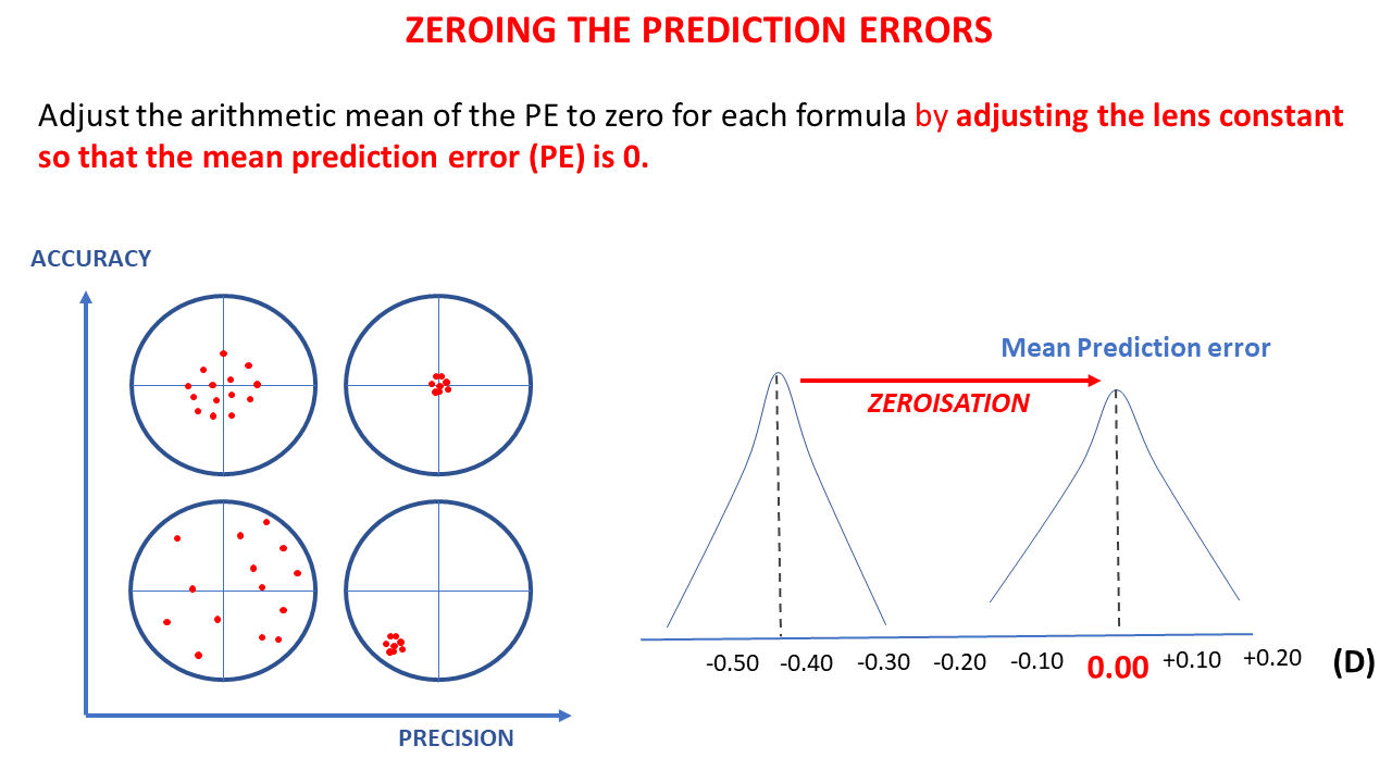
The optimization procedure aims to enhance the accuracy of an IOL power calculation formula for a particular type of IOL. It is indicated when the formula’s average prediction error is significantly different from zero, which implies that the formula exhibits a systematic bias.
This optimization procedure involves adjusting the value of the IOL constant; the goal is that in subsequent calculations, the formula predicts IOL power values that will lead to an average prediction error centered around zero, eliminating systematic bias.
If the average prediction error of an IOL power formula is not zero for a specific IOL model, it is possible to optimize its constant value ourselves without needing to resort to online services or contacting the designer of the relevant formula, thanks to a simple equation that only requires knowledge of three variables: corneal power, implant power, and refractive prediction error. We will return to this point in Section 6 after laying the foundation for optimization.
2. Calculation of the average prediction error of a formula
For a given pseudophakic eye, the prediction error is the difference between the refraction measured after surgery and the refraction predicted by the power calculation formula. If the postoperative refraction obtained is –1 D while the predicted refraction was 0 D, the prediction error equals -1-0 = -1 D.
When we have sufficient eyes operated on for cataracts with a specific IOL model, we can calculate the prediction error of each eye and the average of these errors. The formula is imperfect if this average prediction error is not zero.
NB: The precision of the formula, on the other hand, depends on the dispersion around the average (zero or non-zero). The standard deviation of the prediction error is an essential variable for evaluating the precision of a formula. It is usually calculated after zeroing the mean prediction error.
3. What is the effect of a variation in an IOL constant?
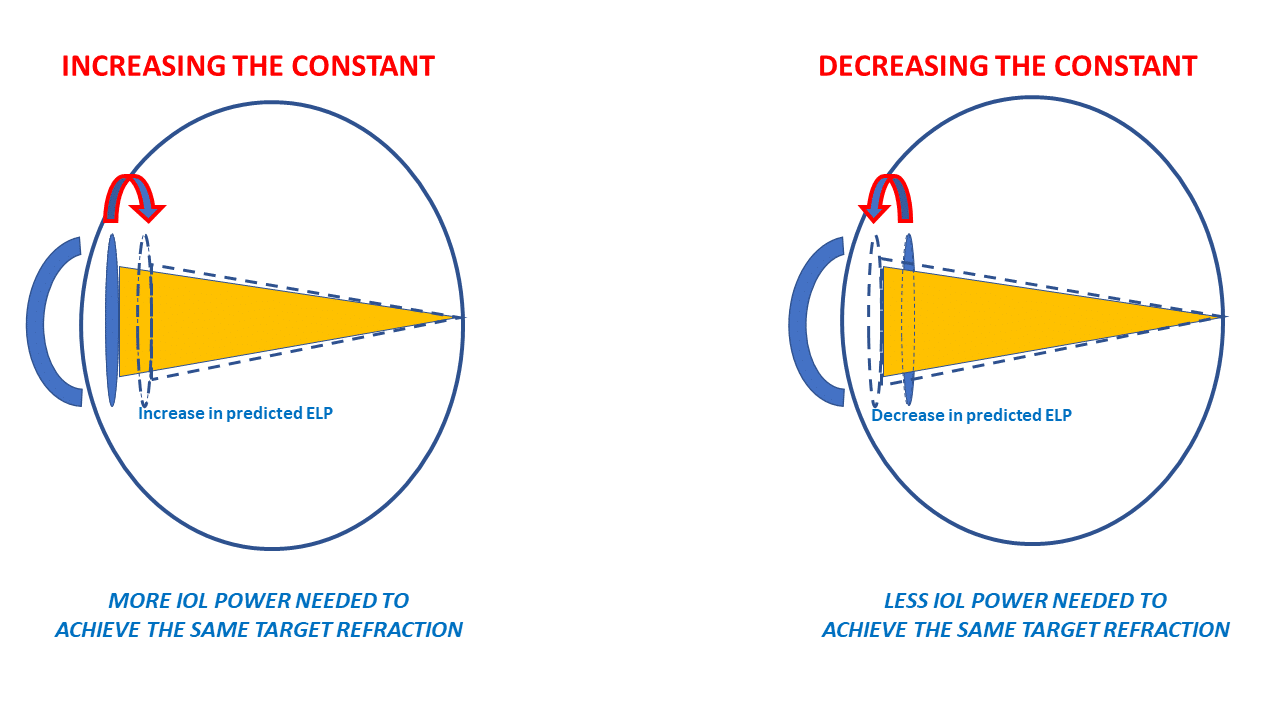
In modern formulas, the constant modification induces a variation in the position of the IOL predicted by the power calculation formula (effective lens prediction: ELP). Modifying a constant means increasing (or decreasing) by a constant increment in the position of all IOLs. Increasing the value of the constant is equivalent to increasing the value of the predicted ELP. Increasing the value of predicted ELP will make the IOL power formula consider that the implant will be positioned further from the cornea. As a result, for the same refractive target to be achieved, the calculation formula will predict a higher power. The corollary of this, meaning the relationships between ELP variations and their impact on refraction for a given IOL power, has been explored on another page.
Hence, the increase of the constant value will be used to compensate for a positive average prediction error (tendency towards postoperative hypermetropization). If a formula constantly increases the predicted position of all implants (towards the retina), it will predict a higher power for the implants for the same target refraction.
If a formula constantly reverses the predicted position of all implants (away from the retina), it will predict a lower power for the implants. The decrease of the constant value will compensate for a negative average prediction error (tendency towards postoperative myopization).
Thus, we can postulate that IOLs with a high constant have a more posterior anatomical and optical position (further from the cornea and closer to the retina ) than IOLs with a lower constant.
The « star » of IOL constants is the A-constant. This constant is historically attached to SRK-type formulas (SRK, SRK II, SRK-T). At this stage, it is crucial to emphasize a crucial point: the meaning of the A-constant is not unequivocal for these formulas, and we will return to this.
The often-used intuitive reasoning is as follows:
• “If with a B-type IOL, I obtain, on average, a slightly hyperopic prediction error with formula X, all I must do is increase the value of my A-constant. For example, if I make an average error of +0.50 D, it should be enough to increase the initial value of the A-constant by about +0.50D to cancel the systematic bias of my formula.”
This reasoning is both correct and incorrect. More specifically, this reasoning was correct at the time of the SRK formula.
This regression formula stipulated that the power of an implant was given by the formula: P = A –2.5 L –0.9 K where A was the formula’s adjustment constant, L the axial length, and K the corneal power.
Modulating the A-constant upward or downward would induce an identical value increment for all powers predicted by the SRK formula. This increment in IOL power was proportional to the mean prediction error to compensate for (+/- 1D of IOL power results in a change of about +/-0.67 D in the refraction at spectacle plane).
With the emergence of so-called theoretical formulas (the T in the SRK-T formula precisely means « theoretical »), calculating the IOL’s power to induce the desired refraction is based on optical concepts.
Theoretical formulas are based on the vergence formula applied to a simplified eye model (cornea + IOL). The distance between the cornea and the IOL must be predicted before the power of the IOL (intended to induce the targeted refraction) can be calculated. The accuracy of this position prediction determines the accuracy of the formula. These theoretical formulas allow for that in case of a refractive bias (a non-zero prediction error), an increment of the effective position of the IOL can cancel this bias.
This presupposes that when a formula is correct, any reduction observed after changing the IOL model is related to a difference in the position of this new model compared to the old one.
Increasing a constant causes the formula to calculate a higher IOL power and vice versa. But, contrary to intuition, the link between the constant increment and the calculated power increment is indirect, unlike what the A-constant initially meant in the context of the original SRK formula. Therefore, it is necessary to transpose this A-constant from a direct power increment (SRK) to a predicted position increment (SRK-T), and we will delve deeper into this point.
4. The Case of the A-Constant
The SRK formula was derived from a regression analysis evaluating the relationship between the power to be placed, axial length, and keratometry. It introduced the concept of a « constant », the variations of which were directly attributed to the predicted power of the implant by the structure of this regression formula. Adding « 1 » to the A-constant was equivalent to adding one diopter to the power of all implants. As introduced with the SRK formula, the implicit unit of the A-constant was the diopter.
It’s easily noticeable that the values assumed by the A-constants, typically around 118, are significantly higher than those of other constants. Indeed, the constants of the theoretical formulas (SF: Holladay, pACD: HofferQ, a0: Haigis) are like increments in millimeters, which are added or subtracted from the predicted position of the implants according to these formulas. Like these third-generation theoretical formulas, the SRK-T formula uses a constant (also named the A-constant) whose variations now relate to the predicted position of the implant (effective lens position).
For historical reasons, it is not possible to relate the value resulting from the difference between two A-constants to a difference in predicted position. Indeed, to preserve the concept of adjustment by this A-constant and not to destabilize the understanding of current users, the designers of the SRK-T formula established a relationship between the true direct position variable called the “ACDconst” and the A-constant. The ACDconst corresponds to the ELP, that is, the distance separating the cornea from the position of the implant (assuming it were a thin lens). Unsurprisingly, the values taken by ACDconst are of the same order of magnitude as the a0, SF, or pACD constants.
This ACDconst value is systematically predicted with the SRK-T as it corresponds to the position of the implant in each eye to be operated. It is a function of an offset named “o” and a distance “h,” which separates the endothelium and the IOL planes. The value of h for a given eye is predicted based on the corneal radius and axial length (see the original articles ). In the SRK-T formula, the value 3.336 serves as a reference to calculate “o,” the constant increment (offset), equal to ACDconst – 3.336 (in millimeters).
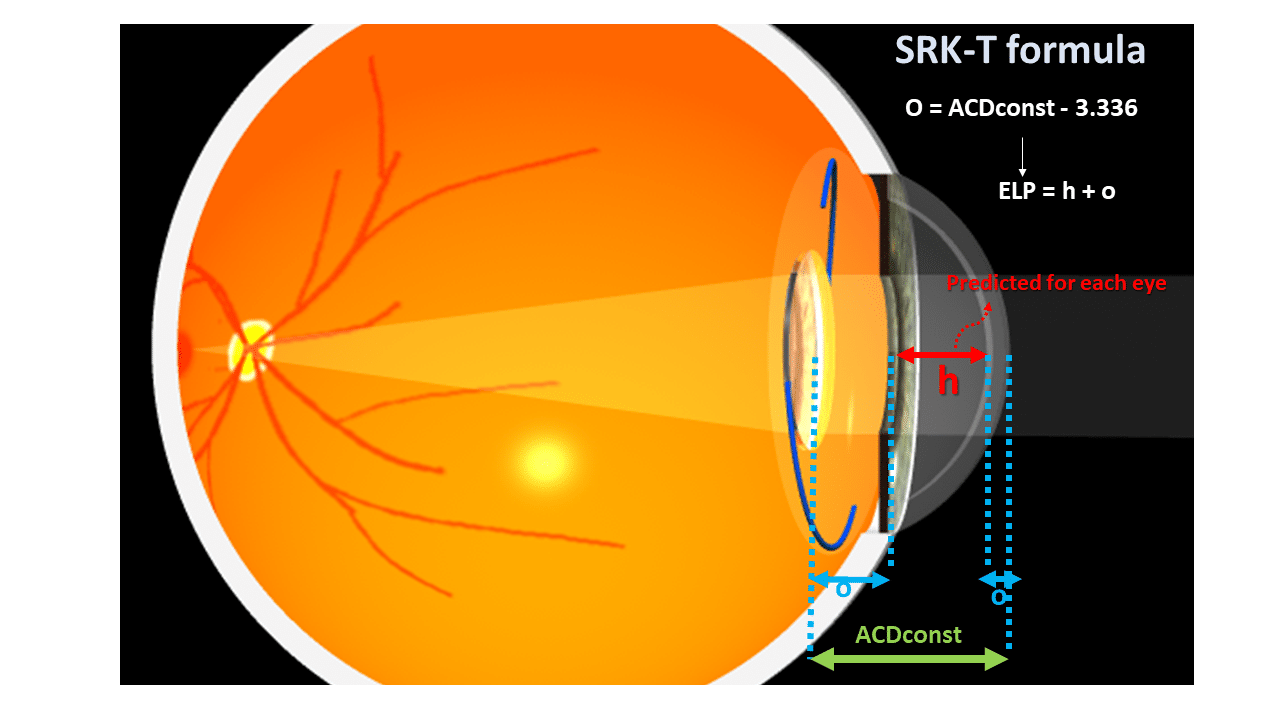
“h” would be the “average” distance to the iris plane from the endothelium, whose average value of 3.336 would be obtained in an “average eye” with a corneal power of 44.18 D and axial length of 23.45 mm (again, these figures come from the equations provided by the original authors of the SRK-T formula in their publication).
This presupposes that the value of o could be deduced from observing the implantation of that IOL implant model in a sufficient number of « average » eyes, whose endothelium-plane distance from the IOL would be, on average, 3.336 mm.
The authors of the SRK-T formula required establishing a link between an ACDconst value (expected implant position) and an A constant value. From their data, the authors built this regression formula:
ACDconst = A constant x 0.62467 – 68.747
(This equation can be solved for the A-constant as a function of ACDconst)
An A-constant of 118.5 corresponds to an ACDconst value of 5.28 mm, a difference (offset) of 1.94 mm with the « average » iris plane (3.336 mm). In the case of the SRK-T formula, this increment is supposed to include corneal thickness.
In a given eye, when the SRK-T formula predicts an implant power value with an A-constant of 118.5, it systematically adds 1.94 mm to h, a distance predicted by a regression formula from the corneal curvature (via the calculation of the corneal sag, which involves an extrapolated corneal diameter) and the axial length of that considered eye. This offset value is comparable to Holladay’s « surgeon factor » (SF) (which does not include corneal thickness, however).
The philosophy of this convoluted approach can be summarized as follows: the value of the offset « o » is specific to the implant, while the anatomical depth of the anterior chamber « h » depends on the eye to be operated. The ACDconst constant is the sum of o (offset specific to the IOL model) and 3.336 (an average anterior chamber depth). For calculating the power of an implant in a given eye, the offset o, calculated as ACDconst – 3.336, is added to the h value predicted for this eye from biometric parameters (axial length and radius of anterior corneal curvature). A regression formula was established by the authors of the SRK-T formula to match the values of ACD-const with the expected values of A-constants for the implants considered: ACDconst = A constant x 0.62467 – 68.747
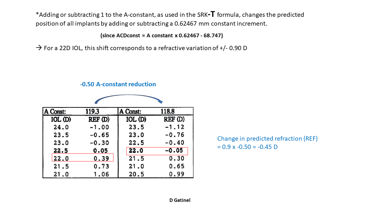
When one is added to the value of the A-constant, the predicted position of the IOL by the SRK-T formula is modified by 0.62467 mm (see equation above). This applies to all calculations, but the crucial point is that, unlike the increment of the A-constant in the SRK (regression) formula, the increment of the A-constant in the SRK-T formula does not result in an identical power increment for all implants.
However, it can be shown that a displacement of about 0.60 mm imposes a refractive variation of about 1 D for an « average » implant power (close to 22D) in an eye of « average » keratometric power (close to 43D); this corroborates the subjective impression that it suffices to increment the A-constant by one unit to compensate for an average prediction error of one unit; however, it must be remembered that this relationship applies only to « average » eyes.
-> Key takeaways are:
*Adding 1 to the A-constant in the SRK formula was equivalent to adding 1D to all predicted powers.
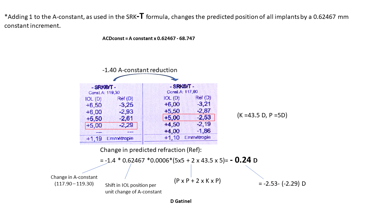
*Adding 1 to the A-constant, as used in the SRK-T formula, changes the predicted position of all implants by a constant increment of 0.62467 mm
This constant incrementing position, however, causes a non-constant increment in the predicted power of the implants: it is important to make these distinctions.
This historical legacy gave the impression that there might be a direct relationship between A-constant variations and predicted IOL power variations. However, the transposition between predicted power modification and predicted ELP modification inspired the generalization of the use of the A-constant to other calculation formulas that can be adjusted to a model whose A-constant value has been determined; these formulas have also established, by regression, the relationship between the A-constant increment and the position increment that these formulas use. This applies, for example, to the Barret Universal II, Kane, PEARL-DGS and some other formulas.
After this laborious but necessary historical detour, we will now discuss how it is possible to calculate the optimal constant of an implant from a data set consisting of the implanted powers, corneal powers, and postoperative refractions.
5 -Adjusting a Constant: Problem Foundations
Let us assume that we have a set of eyes operated with the same implant model, with preoperative biometrics available and known postoperative implant power and refractions. From these refractions, we can easily calculate the average prediction error for a given IOL power formula. Be careful not to confuse prediction error with postoperative refraction: the average prediction error is the average postoperative refraction (average of the spherical equivalent of all operated eyes) only if emmetropia was aimed for in all operated eyes.
If myopic refractions were targeted, the prediction error for these eyes must be calculated as the difference between the achieved refraction and the targeted refraction. If a refraction of -2.50 D was targeted and a refraction of -2.00D was achieved, the prediction error is -2.00-(-2.50) = +0.50 D.
From the data of a set of eyes operated with the same IOL model and the information on preoperative biometrics and implanted powers, we can calculate the ideal constant value for any formula optimized with a single constant – that is, most routinely used. We also need to know the postoperative refractions. Still, this point is inherent to the problem at hand since these refractions are necessary to calculate the mean PE to nullify.
Initially, it is appropriate to select the power calculation formula to optimize and, for each eye in the dataset, determine what the refraction predicted by the formula would be for the power and the model of the implanted IOL. We will choose for that initial calculation the usual or recommended initial constant value for the implanted IOL model.
Then, for each eye, we calculate the difference between the achieved refraction and the refraction predicted by the formula. We then calculate the average (arithmetic mean) of these prediction errors over the entire sample (and if the average prediction error is zero, then optimization will not be necessary !).
If the average prediction error is not zero, it is possible to optimize the constant value ourselves without needing to resort to online services or contacting the designer of the relevant formula, thanks to this simple equation that links these data:
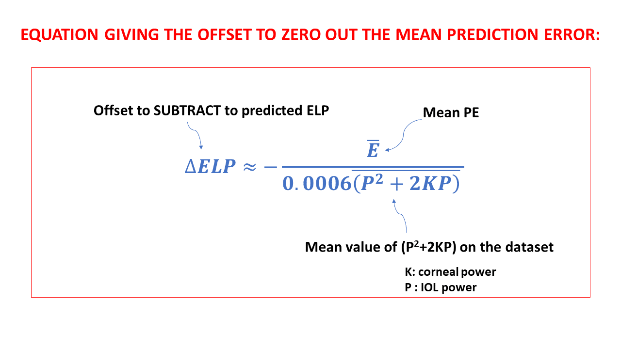
Where ΔELP is the constant increment to be subtracted from the initial constant value, E is the average error, and 0.006 (P^2+2KxP) is the average value of the product 0.0006 (P^2+2KxP) over the dataset.
For instance, in the dataset, if a specific eye has a P value of 22D and a K value of 43D, the product (which is always positive) would be:
0.0006*(22*22+2*22*43)= 1.4256.
This multiplication can be carried out for each individual eye included in the dataset. Following this, it’s straightforward to calculate the average of these product values.
Including a negative sign in front of the fraction in the equation is a direct consequence of the specific method employed when deriving this equation. Further details about this are provided in the subsequent section.
Given the straightforward nature of this equation, which is just based on the average prediction error, the powers of the implanted IOLs, and the corneal powers used by the formula, it is entirely feasible for anyone to compute the necessary constant increment to nullify the average prediction error.
The process leading to the development of this equation will be outlined in the following section.
6) Determining the Constant Increment Necessary for Formula Optimization
We consider the common scenario here, where we are using one of the formulas that are optimized with a single constant:
*A-constant for the SRK-T formula (and formulas that also use the A-constant as a starting point)
*pACD constant for the Hoffer Q formula
*SF constant for the Holladay formula
*a0 constant for the Haigis formula
The refractive system of the pseudophakic eye consists of two lenses: the cornea and the IOL. We first needed to establish a relationship between the change in the IOL’s position (ELP modification) and the impact on the postoperative refraction of the operated eye. The variation in postoperative refraction due to an ELP change logically depends on the power of the cornea and that of the IOL.
We have constructed a theoretical paraxial model that allowed us to obtain the following equation after some calculation steps and a regression step:
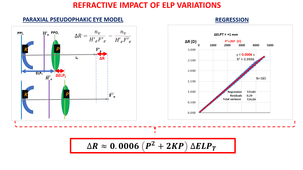
This equation (the derivation of which is available in an Appendix) has been discussed on another page, and will be discussed in an annex to keep this train of thought going. Once the relationship between refractive variation and position variation for a corneal power K and an IOL power P has been established, the following reasoning can be carried out:
If the average prediction error is E on a sample of N eyes, the “total error” on that set is equal to the product of N by E. It is equal to the sum of the prediction errors of all N eyes. This sum will also be zero if the mean prediction error is null.
Total E= N x E
Our task is to bring Total E to null.
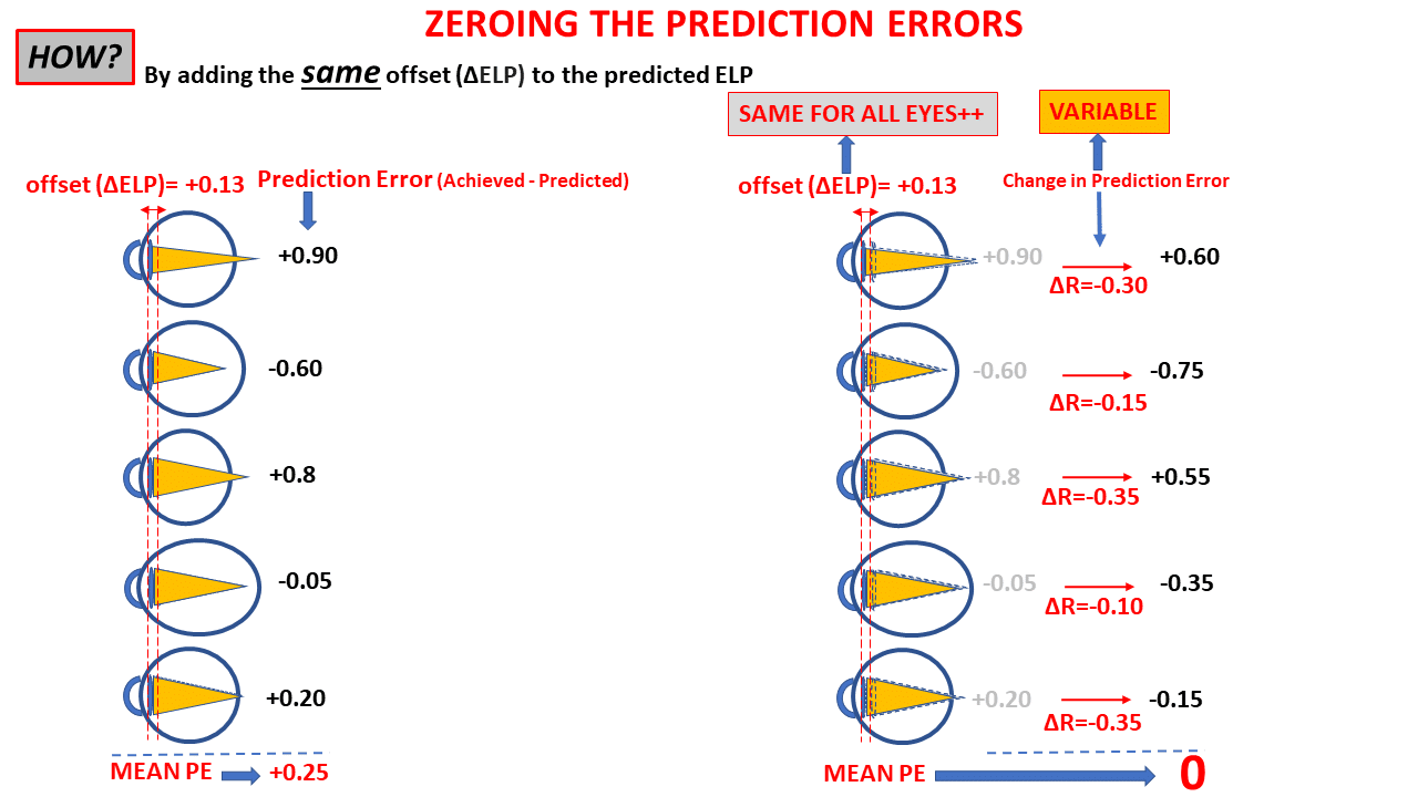
The next task is to determine the value of ΔELP such that the sum of the prediction errors after refraction changes (caused by ΔELP change in ELP) is null. This will happen if the sum of the refractive changes ΔR on the set (after each of the IOLs « moves » by the same distance ΔELP) equals: – N x E:
We can write this as ΣN ΔR = -N x E.
Since for each eye, we have shown that ΔR=ΔELP x 0.0006 x (P^2+2KP), then:
ΣN 〖ΔELP x 0.0006 x (P^2+2KP)〗 = -N x E
We can solve this equation for ΔELP :
ΔELP=(-N x E) / (ΣN 〖 0.0006 x (P^2+2KP)〗)
As (P^2+2KP)/N= P^2+2KP (the “bar” over an expression means that its average value is considered), dividing the fraction by N leads to the following equation:
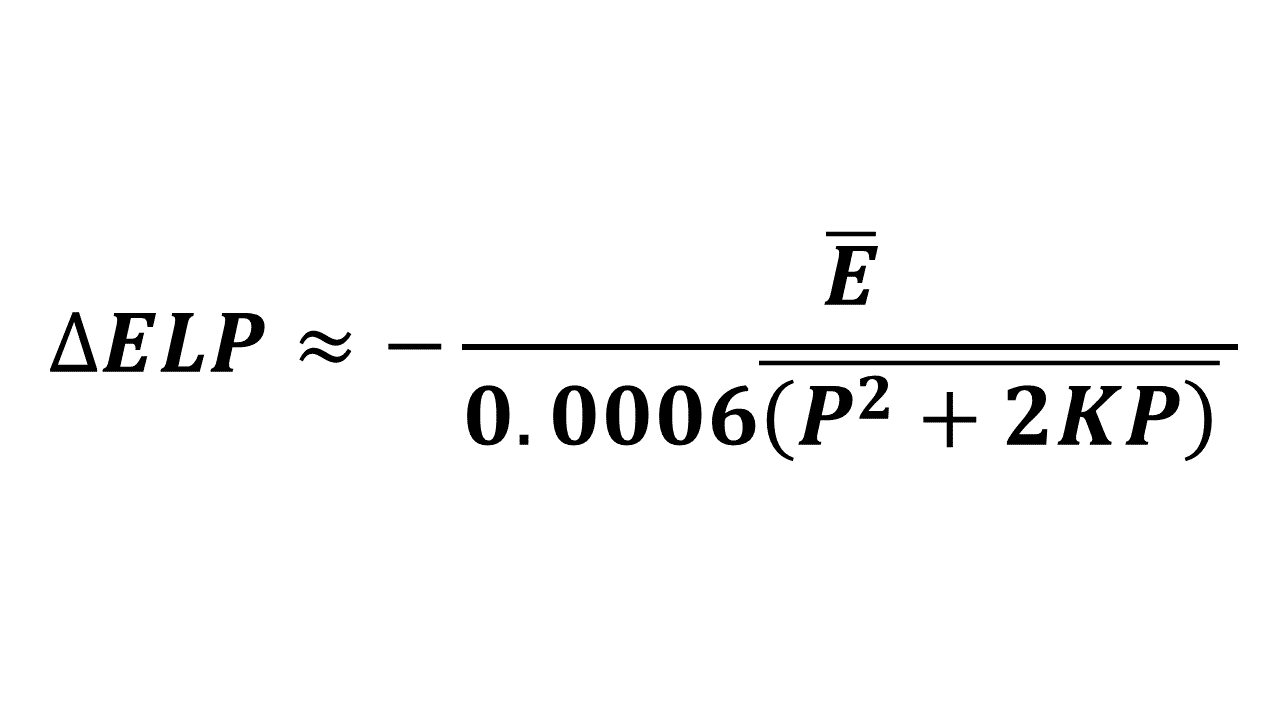
To ensure that a positive prediction error is offset by a positive increment and a negative increment offsets a negative prediction error, it is appropriate to subtract the ΔELP value calculated by this formula from the original constant value.
Let’s assume that E = -0.35 D and 0.006 (P^2+2KxP) = 1.456. Then, ΔELP = – (-0.35/1.456) = 0.241 mm. Depending on the considered IOL power formula, this value can be subtracted from the initial a0, SF, pACD, or Aconst values.
Let’s now assume that ΔELP = -0.25, and the initial constant is 2: the updated constant should be 2-(-0.25) = 2.25.
When E is negative (myopic error), ΔELP is positive: subtracting it reduces the value of the predicted ELP. As expected, this will reduce the calculated power of the implants as they are now all predicted to be at a greater distance from the retina with the same offset (ΔELP).
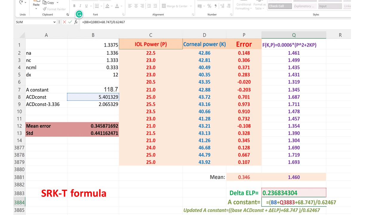
These calculation steps are easily implementable in a simplified format in a spreadsheet, as shown below for the SRK-T formula (the negative sign of the fraction has been removed, then the calculated ΔELP can be added to the initial constant value)
This methodology can be employed iteratively by attributing the residual mean error to the variable E until the reduction in residual error by accumulating the consecutive ELP increments is deemed satisfactory.
The benefit of our approach is that it restricts the necessary calculations to two or three to achieve a mean error value that is as close to zero as possible.
Our methodology can also be used to optimize unpublished formulas like the Barrett Universal II, Hill-RBF, and Kane. These formulas allow surgeons to incorporate the SRK/T optimized A-constant in their computations.
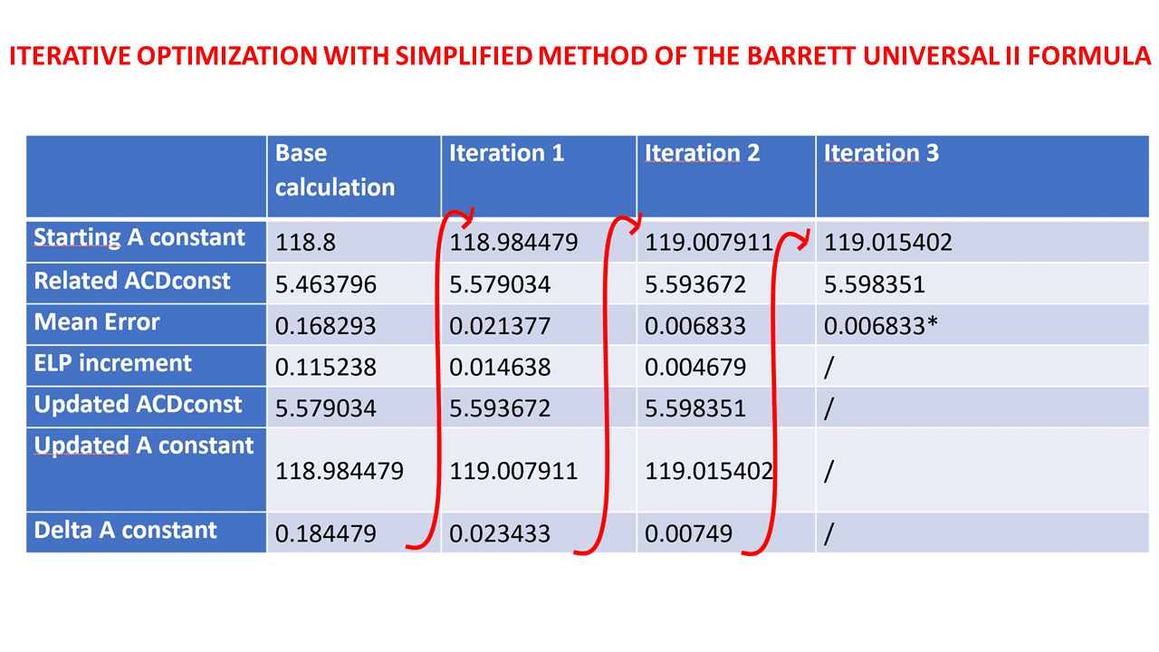
We utilized a dataset of eyes implanted with the Finevision IOL (comprising 3878 eyes) to adjust the IOL constant for the BUII formula via its online calculator. We conducted an initial calculation iteration with a base A-constant of 118.8, sourced from the IOLcon website. We computed the minus ΔELP using the above equation. We added it to the base ACDconst value derived from the A-constant using the linear transformation described above to get the updated ACDconst value. Subsequently, we figured out the revised A constant using a reverse transformation. We executed two more rounds of calculations, each respectively employing the first and second reduced ME values, to observe the mean error’s progression:
7) Annex: Impact of ELP variation on the refraction of the pseudophakic eye
To establish the equation that allows one to nullify the prediction error of an implant power calculation formula, we had to provide an approximation of the refractive impact of an IOL’s movement according to its power and the power of the cornea.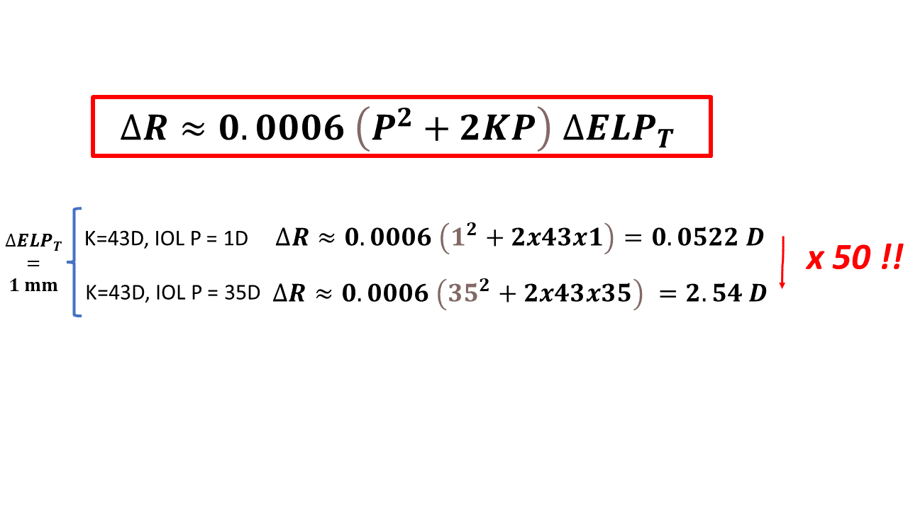
*It can be inferred that the major determinant is the IOL’s power. A simple calculation reveals that for the same movement, there is a factor close to 50 between the refractive variation induced by an implant of 1D vs. 35 D.
This significant discrepancy implies that the nullification of prediction error (PE) in an implant calculation formula is nearly autonomous of eyes receiving low-power implants. These observations indicate that adjusting a single constant is not the most effective approach for enhancing the refractive precision of a formula on extremely elongated eyes, where the PE isn’t derived from an incorrect prediction of the effective lens position (ELP).
*The impact of keratometry is secondary, but it cannot be neglected as it multiplies the power of the IOL. However, in comparison, the variations in the K variable are less significant than those of P.
*For an average power implant (22D) and an average power cornea (44D), it can be established that P^2+2K*P is close to 5*P^2 (as 44= 2x 22). Thus, for average biometric values, ΔR=0.0006x5P^2=0.003P^2. We get a value close to 1.45 D for the refractive change induced by a 1 mm movement for a 22 D implant.
* An addition of 1 to the A-constant is equivalent to a backward IOL movement of 0.62467 mm ( this number is involved in the conversion between ACDconst and A-constant, see above). Therefore, the refractive variation of the pseudophakic eye (with IOL power of 22 D) would be approximately 0.62467 x 1.45 = 0.90 D. After the conversion formula between ACDconst and A-constant, this gives an impression of « one to one » between the increment of 1 of the A-constant and the postoperative refraction increment for IOLs within this « average » power range.
This is why the use of the A-constant has remained popular! (« if my average error is -0.5D, I just need to reduce my constant by a value close to 0.50D »; or : « if I want to compensate for an expected refractive error of 1D, I can increase my A-constant by 1 »).
*For low-power implants, the impact of the constant variation is much lower (the approximation reported above should not be used, which is only valid for IOLs with a power close to 22D). Using our general formula to estimate the impact of the change in A-constant is appropriate.
The average thickness of pseudophakic implants of 22 D is approximately 1 mm. Notably, solely the optic design can cause the effective position of the implant (position of the principal object plane) to fluctuate by this measure between a convex-planar and planar-convex design. This implies that variations in design for that power could lead to a refractive discrepancy of around +/-0.7D (half of 1.45 D).
In real-world applications, most designs range between a symmetric form and a planar-convex form (to mitigate positive spherical aberration), leading to an uncertainty of about half of +/-0.7D ( +/-0.35D). Interestingly, this is commensurate with the mean prediction errors observed when adjustment is necessary for new implant models.
Any Question or Comment? Please ask below.
You are most welcome, thank you for your interest in this topic!
Thank you very much for your explanation.
You are a real genius